How to create a choroplath map in R

Author

Niclas

Published

August 24, 2023

Now and then, you come across choropleth maps presented as animated graphics, like on /r/dataisbeautiful. Personally, I’m not so interested in the end result, but rather in the process that leads to the result. This blog post demonstrates how to create an animated GIF of a choropleth map using R.

Most examples on the internet showcase choropleth maps of either the United States or the European Union. However, the majority of the world’s population does not reside in the United States, nor are they solely interested in international-scale data. Consequently, I’ve chosen to provide an example concerning the precipitation in the German state of Brandenburg since 2015. We will compare the average precipitation in each district to the overall mean precipitation of the reference period. As climatic patterns exhibit seasonal variations, we will calculate the monthly average to determine whether a particular month has experienced above or below average rainfall. Adhering to the convention, we will employ a 30-year period to compute climate normals as the mean and select the time frame from January 1970 to December 1999 as the reference period.

Step 1: Data aquisition

The geographical data

Each German state is divided into various districts, necessitating data that provides a high-resolution representation of the administrative boundaries. The website gadm.org provides open data that suits our requirements, and their license permits its use under a CC-BY license. We acquire the geojson-file for the level 2 subdistricts from the website and then proceed to open it within R.

This process is quite straightforward, requiring just a few lines of code in R: 31b8e172-b470-440e-83d8-e6b185028602:dAB5AHAAZQA6AE8AUQBCAGoAQQBHAEkAQQBOAHcAQQA1AEEARwBVAEEATgBnAEIAagBBAEMAMABBAE8AQQBBADQAQQBEAGcAQQBaAEEAQQB0AEEARABRAEEAWQBRAEEAdwBBAEcAVQBBAEwAUQBBADUAQQBHAE0AQQBPAFEAQgBpAEEAQwAwAEEAWgBnAEIAbQBBAEQAWQBBAE4AdwBCAGoAQQBHAFEAQQBOAEEAQQB3AEEARABRAEEAWgBRAEEAMgBBAEQAQQBBAAoAcABvAHMAaQB0AGkAbwBuADoATQBRAEEANQBBAEQAQQBBAE8AQQBBAD0ACgBwAHIAZQBmAGkAeAA6AAoAcwBvAHUAcgBjAGUAOgBZAEEAQgBnAEEARwBBAEEAZQB3AEIANwBBAEgASQBBAGYAUQBCADkAQQBBAG8AQQBiAEEAQgBwAEEARwBJAEEAYwBnAEIAaABBAEgASQBBAGUAUQBBAG8AQQBIAE0AQQBaAGcAQQBwAEEAQwBBAEEAQwBnAEIAegBBAEcAWQBBAFgAdwBCAG4AQQBHAFUAQQBjAGcAQgB0AEEARwBFAEEAYgBnAEIANQBBAEMAQQBBAFAAQQBBAHQAQQBDAEEAQQBjAHcAQgAwAEEARgA4AEEAYwBnAEIAbABBAEcARQBBAFoAQQBBAG8AQQBDAEkAQQBMAHcAQgB3AEEARwBFAEEAZABBAEIAbwBBAEYAOABBAGQAQQBCAHYAQQBGADgAQQBaAGcAQgBwAEEARwB3AEEAWgBRAEEAdgBBAEcAYwBBAFkAUQBCAGsAQQBHADAAQQBOAEEAQQB4AEEARgA4AEEAUgBBAEIARgBBAEYAVQBBAFgAdwBBAHkAQQBDADQAQQBhAGcAQgB6AEEARwA4AEEAYgBnAEEAaQBBAEMAawBBAEMAZwBBAEsAQQBDAE0AQQBJAEEAQgB6AEEARwBVAEEAYgBBAEIAbABBAEcATQBBAGQAQQBBAGcAQQBIAFEAQQBhAEEAQgBsAEEAQwBBAEEAYwB3AEIAMABBAEcARQBBAGQAQQBCAGwAQQBDAEEAQQBRAGcAQgB5AEEARwBFAEEAYgBnAEIAawBBAEcAVQBBAGIAZwBCAGkAQQBIAFUAQQBjAGcAQgBuAEEAQwBBAEEAYgB3AEIAbQBBAEMAQQBBAFIAdwBCAGwAQQBIAEkAQQBiAFEAQgBoAEEARwA0AEEAZQBRAEEAZwBBAEcAWQBBAGMAZwBCAHYAQQBHADAAQQBJAEEAQgAwAEEARwBnAEEAWgBRAEEAZwBBAEgATQBBAGEAQQBCAGgAQQBIAEEAQQBaAFEAQgBtAEEARwBrAEEAYgBBAEIAbABBAEEAbwBBAGMAdwBCAG0AQQBGADgAQQBZAGcAQgB5AEEARwBFAEEAYgBnAEIAawBBAEcAVQBBAGIAZwBCAGkAQQBIAFUAQQBjAGcAQgBuAEEAQwBBAEEAUABBAEEAdABBAEMAQQBBAFoAZwBCAHAAQQBHAHcAQQBkAEEAQgBsAEEASABJAEEASwBBAEIAegBBAEcAWQBBAFgAdwBCAG4AQQBHAFUAQQBjAGcAQgB0AEEARwBFAEEAYgBnAEIANQBBAEMAdwBBAEkAQQBCAE8AQQBFAEUAQQBUAFEAQgBGAEEARgA4AEEATQBRAEEAZwBBAEQAMABBAFAAUQBBAGcAQQBDAEkAQQBRAGcAQgB5AEEARwBFAEEAYgBnAEIAawBBAEcAVQBBAGIAZwBCAGkAQQBIAFUAQQBjAGcAQgBuAEEAQwBJAEEASwBRAEEASwBBAEcAQQBBAFkAQQBCAGcAQQBBAD0APQAKAHMAdQBmAGYAaQB4ADoA:31b8e172-b470-440e-83d8-e6b185028602

The meteorological data

The German meteorological service, Deutscher Wetterdienst (DWD), publishes meteorological and climate data in Germany under a permissive license. This data is accessible through the DWD’s Server. While manually downloading the data is a bit cumbersome, we have opted to utilize the RDWD package to streamline the process of selecting the appropriate data. However, selecting the correct meteorological station and their corresponding ID is crucial.

The climate data stations are documented in a txt-file, which we read and store for all weather stations in Brandenburg using the read_table function from the readr package. This function is capable of directly reading URLs, allowing us to retrieve the data from the web without intermediaries. Yet, our interest is limited to stations with data available in the climate normal period of January 1970 to December 1999, and we apply data filtering using the dplyr package.

Following the station selection, we employ the selectDWD function from the rdwd package to choose the relevant stations on the server and subsequently download them. The code for this process is relatively straightforward:

```{r}
library(readr)
library(lubridate)

climate_normal_start <- ymd(19700101)
climate_normal_end <- ymd(19991231)

stations_germany <- read_table("https://opendata.dwd.de/climate_environment/CDC/observations_germany/climate/monthly/kl/historical/KL_Monatswerte_Beschreibung_Stationen.txt",  col_types = cols(Stationshoehe = col_skip(), Stationsname = col_skip()))

# select the stations in Brandenburg
stations_brandenburg <- stations_germany %>%
  mutate(von_datum = ymd(von_datum), bis_datum = ymd(bis_datum)) %>%
  filter(Bundesland == "Brandenburg" & von_datum <= climate_normal_start & bis_datum >= climate_normal_end)

# Download the meteorological data
urls <- selectDWD(id=stations_subdivisions$station_id, res = "monthly", var = "kl", per = "hr")
meteo_data_raw <- dataDWD(urls)
meteo_data <- bind_rows(meteo_data_raw) %>%
  mutate(month_measurement = as_date(MESS_DATUM), precipitation = MO_RR) %>%
  select(STATIONS_ID, month_measurement, precipitation) %>%
  rename(station_id = STATIONS_ID) 
```

The data for each station is stored individually on the server, and the dataDWD function returns a list of data frames. We use the rbind function to concatenate these data frames, creating a single data frame. Specifically, we focus on the MO_RR column, which represents precipitation measurements at each station. We select this column along with the corresponding month of measurement and the station’s unique ID.

The details regarding the data frame stations_subsdivision will be elaborated in the following section.

Step 2: Select the district of each meteorological station

In the next step we have to combine the data our geographical data with our meteorological data.To accomplish this, we create a data frame that includes the station’s ID and its corresponding district information.

The weather station’s coordinates are provided as longitude and latitude, while the subdistricts contain a geometry column that defines the boundary of each district as a polygon. Given that the districts form a partition of Brandenburg’s surface, we can determine whether a weather station’s location falls within a particular polygon using the st_contains function.

This process yields a temporary data frame named stations_subdivisions, which establishes a mapping between the weather station’s ID and the corresponding district. 31b8e172-b470-440e-83d8-e6b185028602:dAB5AHAAZQA6AE8AUQBCAGoAQQBHAEkAQQBOAHcAQQA1AEEARwBVAEEATgBnAEIAagBBAEMAMABBAE8AQQBBADQAQQBEAGcAQQBaAEEAQQB0AEEARABRAEEAWQBRAEEAdwBBAEcAVQBBAEwAUQBBADUAQQBHAE0AQQBPAFEAQgBpAEEAQwAwAEEAWgBnAEIAbQBBAEQAWQBBAE4AdwBCAGoAQQBHAFEAQQBOAEEAQQB3AEEARABRAEEAWgBRAEEAMgBBAEQAQQBBAAoAcABvAHMAaQB0AGkAbwBuADoATgBRAEEANQBBAEQATQBBAE8AUQBBAD0ACgBwAHIAZQBmAGkAeAA6AAoAcwBvAHUAcgBjAGUAOgBZAEEAQgBnAEEARwBBAEEAZQB3AEIANwBBAEgASQBBAGYAUQBCADkAQQBBAG8AQQBJAHcAQQBnAEEARQBNAEEAYgB3AEIAdABBAEgAQQBBAGQAUQBCADAAQQBHAFUAQQBJAEEAQgAwAEEARwBnAEEAWgBRAEEAZwBBAEcATQBBAGIAQQBCAHAAQQBHADAAQQBZAFEAQgAwAEEARwBVAEEASQBBAEIAdQBBAEcAOABBAGMAZwBCAHQAQQBHAEUAQQBiAEEAQgB6AEEAQwBBAEEAWgBnAEIAdgBBAEgASQBBAEkAQQBCAGwAQQBHAEUAQQBZAHcAQgBvAEEAQwBBAEEAYgBRAEIAdgBBAEcANABBAGQAQQBCAG8AQQBDAEEAQQBZAFEAQgB1AEEARwBRAEEASQBBAEIAegBBAEgAVQBBAFkAZwBCAGsAQQBHAGsAQQBkAGcAQgBwAEEASABNAEEAYQBRAEIAdgBBAEcANABBAEwAZwBBAGcAQQBGAGMAQQBaAFEAQQBnAEEARwBNAEEAYgB3AEIAdABBAEgAQQBBAGQAUQBCADAAQQBHAFUAQQBJAEEAQgAwAEEARwBnAEEAWgBRAEEAZwBBAEcAMABBAFoAUQBCAGgAQQBHADQAQQBMAEEAQQBLAEEAQwBNAEEASQBBAEIAMABBAEcAZwBBAFoAUQBBAGcAQQBIAE0AQQBkAEEAQgBoAEEARwA0AEEAWgBBAEIAaABBAEgASQBBAFoAQQBBAGcAQQBHAFUAQQBjAGcAQgB5AEEARwA4AEEAYwBnAEEAZwBBAEcAOABBAFoAZwBBAGcAQQBIAFEAQQBhAEEAQgBsAEEAQwBBAEEAYgBRAEIAbABBAEcARQBBAGIAZwBBAHMAQQBDAEEAQQBZAFEAQgB1AEEARwBRAEEASQBBAEIAMABBAEcAZwBBAFoAUQBBAGcAQQBHADQAQQBkAFEAQgB0AEEARwBJAEEAWgBRAEIAeQBBAEMAQQBBAGIAdwBCAG0AQQBDAEEAQQBjAHcAQgAwAEEARwBFAEEAZABBAEIAcABBAEcAOABBAGIAZwBCAHoAQQBDAEEAQQBaAGcAQgB2AEEASABJAEEASQBBAEIAbABBAEcARQBBAFkAdwBCAG8AQQBDAEEAQQBaAEEAQgBwAEEASABNAEEAZABBAEIAeQBBAEcAawBBAFkAdwBCADAAQQBDADQAQQBDAGcAQgBqAEEARwB3AEEAYQBRAEIAdABBAEcARQBBAGQAQQBCAGwAQQBGADgAQQBiAGcAQgB2AEEASABJAEEAYgBRAEIAaABBAEcAdwBBAGMAdwBBAGcAQQBEAHcAQQBMAFEAQQBnAEEARwAwAEEAWgBRAEIAMABBAEcAVQBBAGIAdwBCAGYAQQBHAFEAQQBZAFEAQgAwAEEARwBFAEEASQBBAEEAbABBAEQANABBAEoAUQBBAEsAQQBDAEEAQQBJAEEAQgBtAEEARwBrAEEAYgBBAEIAMABBAEcAVQBBAGMAZwBBAG8AQQBHADAAQQBiAHcAQgB1AEEASABRAEEAYQBBAEIAZgBBAEcAMABBAFoAUQBCAGgAQQBIAE0AQQBkAFEAQgB5AEEARwBVAEEAYgBRAEIAbABBAEcANABBAGQAQQBBAGcAQQBEADQAQQBQAFEAQQBnAEEARwBNAEEAYgBBAEIAcABBAEcAMABBAFkAUQBCADAAQQBHAFUAQQBYAHcAQgB1AEEARwA4AEEAYwBnAEIAdABBAEcARQBBAGIAQQBCAGYAQQBIAE0AQQBkAEEAQgBoAEEASABJAEEAZABBAEEAZwBBAEMAWQBBAEkAQQBCAHQAQQBHADgAQQBiAGcAQgAwAEEARwBnAEEAWAB3AEIAdABBAEcAVQBBAFkAUQBCAHoAQQBIAFUAQQBjAGcAQgBsAEEARwAwAEEAWgBRAEIAdQBBAEgAUQBBAEkAQQBBADgAQQBEADAAQQBJAEEAQgBqAEEARwB3AEEAYQBRAEIAdABBAEcARQBBAGQAQQBCAGwAQQBGADgAQQBiAGcAQgB2AEEASABJAEEAYgBRAEIAaABBAEcAdwBBAFgAdwBCAGwAQQBHADQAQQBaAEEAQQBwAEEAQwBBAEEASgBRAEEAKwBBAEMAVQBBAEMAZwBBAGcAQQBDAEEAQQBiAFEAQgAxAEEASABRAEEAWQBRAEIAMABBAEcAVQBBAEsAQQBCAHQAQQBHADgAQQBiAGcAQgAwAEEARwBnAEEASQBBAEEAOQBBAEMAQQBBAGIAUQBCAHYAQQBHADQAQQBkAEEAQgBvAEEAQwBnAEEAYgBRAEIAdgBBAEcANABBAGQAQQBCAG8AQQBGADgAQQBiAFEAQgBsAEEARwBFAEEAYwB3AEIAMQBBAEgASQBBAFoAUQBCAHQAQQBHAFUAQQBiAGcAQgAwAEEAQwBrAEEASwBRAEEAZwBBAEMAVQBBAFAAZwBBAGwAQQBBAG8AQQBJAEEAQQBnAEEARwBjAEEAYwBnAEIAdgBBAEgAVQBBAGMAQQBCAGYAQQBHAEkAQQBlAFEAQQBvAEEARwAwAEEAYgB3AEIAdQBBAEgAUQBBAGEAQQBBAHMAQQBDAEEAQQBjAHcAQgAxAEEARwBJAEEAWgBBAEIAcABBAEgAWQBBAGEAUQBCAHoAQQBHAGsAQQBiAHcAQgB1AEEAQwBrAEEASQBBAEEAbABBAEQANABBAEoAUQBBAEsAQQBDAEEAQQBJAEEAQgB6AEEASABVAEEAYgBRAEIAdABBAEcARQBBAGMAZwBCAHAAQQBIAE0AQQBaAFEAQQBvAEEARwAwAEEAWgBRAEIAaABBAEcANABBAFgAdwBCAHcAQQBIAEkAQQBaAFEAQgBqAEEARwBrAEEAYwBBAEIAcABBAEgAUQBBAFkAUQBCADAAQQBHAGsAQQBiAHcAQgB1AEEAQwBBAEEAUABRAEEAZwBBAEcAMABBAFoAUQBCAGgAQQBHADQAQQBLAEEAQgB3AEEASABJAEEAWgBRAEIAagBBAEcAawBBAGMAQQBCAHAAQQBIAFEAQQBZAFEAQgAwAEEARwBrAEEAYgB3AEIAdQBBAEMAdwBBAEkAQQBCAHUAQQBHAEUAQQBMAGcAQgB5AEEARwAwAEEASQBBAEEAOQBBAEMAQQBBAFYAQQBCAFMAQQBGAFUAQQBSAFEAQQBwAEEAQwB3AEEAQwBnAEEAZwBBAEMAQQBBAEkAQQBBAGcAQQBDAEEAQQBJAEEAQQBnAEEAQwBBAEEASQBBAEEAZwBBAEMAQQBBAEkAQQBCAHoAQQBHAFUAQQBYAHcAQgB3AEEASABJAEEAWgBRAEIAagBBAEcAawBBAGMAQQBCAHAAQQBIAFEAQQBZAFEAQgAwAEEARwBrAEEAYgB3AEIAdQBBAEMAQQBBAFAAUQBBAGcAQQBIAE0AQQBaAEEAQQBvAEEASABBAEEAYwBnAEIAbABBAEcATQBBAGEAUQBCAHcAQQBHAGsAQQBkAEEAQgBoAEEASABRAEEAYQBRAEIAdgBBAEcANABBAEwAQQBBAGcAQQBHADQAQQBZAFEAQQB1AEEASABJAEEAYgBRAEEAZwBBAEQAMABBAEkAQQBCAFUAQQBGAEkAQQBWAFEAQgBGAEEAQwBrAEEASQBBAEEAdgBBAEMAQQBBAGMAdwBCAHgAQQBIAEkAQQBkAEEAQQBvAEEARwA0AEEASwBBAEEAcABBAEMAawBBAEwAQQBBAEsAQQBDAEEAQQBJAEEAQQBnAEEAQwBBAEEASQBBAEEAZwBBAEMAQQBBAEkAQQBBAGcAQQBDAEEAQQBJAEEAQQBnAEEARwA0AEEAZABRAEIAdABBAEcASQBBAFoAUQBCAHkAQQBGADgAQQBjAHcAQgAwAEEARwBFAEEAZABBAEIAcABBAEcAOABBAGIAZwBCAHoAQQBDAEEAQQBQAFEAQQBnAEEARwA0AEEASwBBAEEAcABBAEMAdwBBAEMAZwBBAGcAQQBDAEEAQQBJAEEAQQBnAEEAQwBBAEEASQBBAEEAZwBBAEMAQQBBAEkAQQBBAGcAQQBDAEEAQQBJAEEAQQBwAEEAQQBvAEEAWQBBAEIAZwBBAEcAQQBBAAoAcwB1AGYAZgBpAHgAOgA=:31b8e172-b470-440e-83d8-e6b185028602

In the last step we do a left join, so our meterological data now contains the information about the station’s district.

Step 3: Computations

To begin, we calculate the mean, standard error for each mean, and the number of stations within each district during the reference period for the climate from January 1970 to December 1999. This analysis is performed using the summarise function from the dplyr package.

The process is carried out using the following R code: 31b8e172-b470-440e-83d8-e6b185028602:dAB5AHAAZQA6AE8AUQBCAGoAQQBHAEkAQQBOAHcAQQA1AEEARwBVAEEATgBnAEIAagBBAEMAMABBAE8AQQBBADQAQQBEAGcAQQBaAEEAQQB0AEEARABRAEEAWQBRAEEAdwBBAEcAVQBBAEwAUQBBADUAQQBHAE0AQQBPAFEAQgBpAEEAQwAwAEEAWgBnAEIAbQBBAEQAWQBBAE4AdwBCAGoAQQBHAFEAQQBOAEEAQQB3AEEARABRAEEAWgBRAEEAMgBBAEQAQQBBAAoAcABvAHMAaQB0AGkAbwBuADoATgB3AEEAdwBBAEQAQQBBAE0AZwBBAD0ACgBwAHIAZQBmAGkAeAA6AAoAcwBvAHUAcgBjAGUAOgBZAEEAQgBnAEEARwBBAEEAZQB3AEIANwBBAEgASQBBAGYAUQBCADkAQQBBAG8AQQBJAEEAQgB5AEEARwBVAEEAWQB3AEIAbABBAEcANABBAGQAQQBCAGYAQQBHAFEAQQBZAFEAQgAwAEEARwBFAEEASQBBAEEAOABBAEMAMABBAEkAQQBCAHQAQQBHAFUAQQBkAEEAQgBsAEEARwA4AEEAWAB3AEIAawBBAEcARQBBAGQAQQBCAGgAQQBDAEEAQQBKAFEAQQArAEEAQwBVAEEAQwBnAEEAZwBBAEMAQQBBAFoAZwBCAHAAQQBHAHcAQQBkAEEAQgBsAEEASABJAEEASwBBAEIAdABBAEcAOABBAGIAZwBCADAAQQBHAGcAQQBYAHcAQgB0AEEARwBVAEEAWQBRAEIAegBBAEgAVQBBAGMAZwBCAGwAQQBHADAAQQBaAFEAQgB1AEEASABRAEEASQBBAEEAKwBBAEQAMABBAEkAQQBCAHoAQQBIAFEAQQBZAFEAQgB5AEEASABRAEEAWAB3AEIAeQBBAEcAVQBBAFkAdwBCAGwAQQBHADQAQQBkAEEAQgBmAEEASABBAEEAWgBRAEIAeQBBAEcAawBBAGIAdwBCAGsAQQBDAGsAQQBJAEEAQQBsAEEARAA0AEEASgBRAEEASwBBAEMAQQBBAEkAQQBCAHQAQQBIAFUAQQBkAEEAQgBoAEEASABRAEEAWgBRAEEAbwBBAEcAMABBAGIAdwBCAHUAQQBIAFEAQQBhAEEAQQBnAEEARAAwAEEASQBBAEIAdABBAEcAOABBAGIAZwBCADAAQQBHAGcAQQBLAEEAQgB0AEEARwA4AEEAYgBnAEIAMABBAEcAZwBBAFgAdwBCAHQAQQBHAFUAQQBZAFEAQgB6AEEASABVAEEAYwBnAEIAbABBAEcAMABBAFoAUQBCAHUAQQBIAFEAQQBLAFEAQQBzAEEAQQBvAEEASQBBAEEAZwBBAEMAQQBBAEkAQQBBAGcAQQBDAEEAQQBJAEEAQQBnAEEAQwBBAEEAZQBRAEIAbABBAEcARQBBAGMAZwBBAGcAQQBEADAAQQBJAEEAQgA1AEEARwBVAEEAWQBRAEIAeQBBAEMAZwBBAGIAUQBCAHYAQQBHADQAQQBkAEEAQgBvAEEARgA4AEEAYgBRAEIAbABBAEcARQBBAGMAdwBCADEAQQBIAEkAQQBaAFEAQgB0AEEARwBVAEEAYgBnAEIAMABBAEMAawBBAEsAUQBBAGcAQQBDAFUAQQBQAGcAQQBsAEEAQQBvAEEASQBBAEEAZwBBAEcAYwBBAGMAZwBCAHYAQQBIAFUAQQBjAEEAQgBmAEEARwBJAEEAZQBRAEEAbwBBAEcAMABBAGIAdwBCAHUAQQBIAFEAQQBhAEEAQQBzAEEAQwBBAEEAZQBRAEIAbABBAEcARQBBAGMAZwBBAHMAQQBDAEEAQQBjAHcAQgAxAEEARwBJAEEAWgBBAEIAcABBAEgAWQBBAGEAUQBCAHoAQQBHAGsAQQBiAHcAQgB1AEEAQwBrAEEASQBBAEEAbABBAEQANABBAEoAUQBBAEsAQQBDAEEAQQBJAEEAQgB6AEEASABVAEEAYgBRAEIAdABBAEcARQBBAGMAZwBCAHAAQQBIAE0AQQBaAFEAQQBvAEEASABJAEEAWgBRAEIAagBBAEcAVQBBAGIAZwBCADAAQQBGADgAQQBiAFEAQgBsAEEARwBFAEEAYgBnAEEAZwBBAEQAMABBAEkAQQBCAHQAQQBHAFUAQQBZAFEAQgB1AEEAQwBnAEEAYwBBAEIAeQBBAEcAVQBBAFkAdwBCAHAAQQBIAEEAQQBhAFEAQgAwAEEARwBFAEEAZABBAEIAcABBAEcAOABBAGIAZwBBAHMAQQBDAEEAQQBiAGcAQgBoAEEAQwA0AEEAYwBnAEIAdABBAEMAQQBBAFAAUQBBAGcAQQBGAFEAQQBVAGcAQgBWAEEARQBVAEEASwBRAEEAcwBBAEMAQQBBAGIAZwBBAGcAQQBEADAAQQBJAEEAQgB1AEEAQwBnAEEASwBRAEEAcABBAEEAbwBBAFkAQQBCAGcAQQBHAEEAQQAKAHMAdQBmAGYAaQB4ADoA:31b8e172-b470-440e-83d8-e6b185028602

The number of stations and the standard error for the mean are just for the one, who sits in front of the screen. IThese figures facilitate a better understanding of the data and potential errors. The identical calculation is performed for the recent meteorological data, encompassing measurements since January 2015.

```{r}
 recent_data <- meteo_data %>%
  filter(month_measurement >= start_recent_period) %>%
  mutate(month = month(month_measurement),
         year = year(month_measurement)) %>%
  group_by(month, year, subdivision) %>%
  summarise(recent_mean = mean(precipitation, na.rm = TRUE), n = n())
```

In the final computational step, we determine the relative precipitation \(r_p\) using the formula:

\[ r_p = \frac{p}{\overline{p}}. \]

In this equation, \(p\) represents precipitation, and \(\overline{p}\) signifies the average precipitation. The outcome is a dimensionless value that enables a comparison between a month’s precipitation in a specific region and the reference period’s precipitation within the climate timeframe. For instance, \(r_p = 1.1\) indicates that the precipitation during this month was 10% higher than the average.

The provided R code computes the relative score and integrates it into the shapefile.

```{r}
# compute the relative precipitation for each district and
# each month since Jan 2015.
scores_subdivisions <- left_join(recent_data, climate_normals) %>%
  ungroup() %>%
  mutate(relative_precipitation = round(recent_mean / mean_precipitation , 1),
         month = make_date(year, month, 1)) %>%
  select(subdivision,month,  relative_precipitation)


sf_brandenburg_plot <- sf_brandenburg %>%
  mutate(temp_id = 1) %>%
  full_join(expand.grid(temp_id = 1, month = seq(start_recent_period, end_recent_period, by = "month"))) %>%
  left_join(scores_subdivisions, by = c("NAME_2" = "subdivision", "month" = "month")) %>%
  select(-temp_id)
```

Step 4: Create frames for the animation

We aim to construct an animation. The typical choice for creating animations in R is the gganimate package, which, however, has numerous dependencies. Like more often than not, I encountered problems while attempting to install all of these dependencies on my Linux distribution laptop. As a workaround, I devised a solution involving the generation of each frame individually. Subsequently, I developed a small CLI program to merge these frames into a GIF file.

The ggplot2 package provides the geom_sf plot geometry function, streamlining the process of plotting shapefiles.

For every month, we craft a plot using ggplot2 and store it within a local directory named frames.

```{r}
end_recent_period <- max(scores_subdivisions$month)
relative_precipitation_min <- min(scores_subdivisions$relative_precipitation, na.rm = TRUE)
relative_precipitation_max <- max(scores_subdivisions$relative_precipitation, na.rm = TRUE)

for (m in unique(sf_brandenburg_plot$month)) {
  p <- sf_brandenburg_plot %>%
    filter(month == m) %>%
    ggplot() + 
    geom_sf(aes(fill=relative_precipitation)) +
    scale_fill_gradient2(low = "red", high = "darkblue", mid = "green", midpoint = 1, na.value = "grey", 
                        limits = c(relative_precipitation_min, relative_precipitation_max),
                        name = "relative precipitation") + 
    theme_bw() +
    labs(title="Deviation of the precipitation from the mean of 1970 - 1999 \n in Brandenburg, Germany") +
    annotate(geom="label", x = 11.9, y = 51.8, label = paste("Month:", strftime(as_date(m), "%b %Y")), fill="white") +
    xlab("") + 
    ylab("")
  
  ggsave(paste0("/my_path//frames/frame-", strftime(as_date(m), "%Y-%m"), ".png"), p)

}
```

Step 5: Create an animation from the frames

In the last step, I coded a small python programm which uses the libraries Pillow and Python Fire to create a gif file. The source code is relative short:

```{python}
 # Load libraries
 import os
import sys
from PIL import Image
import fire

# define constants
DEFAULT_OUTPUT_PATH = "./"
DOT = "."
SUPPORTED_FORMATS = ("jpeg", ".jpeg", "jpg", ".jpg", ".png", "png")

# define the function to create the output gif.
def combine_to_gif(name:str="output.gif", output_path:str=DEFAULT_OUTPUT_PATH, file_type:str=".png", duration:int=500, print_done:bool=False, *args):
    if output_path == DEFAULT_OUTPUT_PATH:
        output_path = os.getcwd()
    
    try:
        if file_type not in SUPPORTED_FORMATS:
            raise ValueError
        if len(args) == 0:
            args = sys.stdin.read().splitlines() # read from command line
        if len(args) == 0:
            raise ValueError("No images given")
        frames = [Image.open(arg) for arg in args]
        img = frames[0]
        file_path = output_path + "/" + name
        img.save(fp=file_path, format="GIF", append_images=frames,
                 save_all=True, duration=duration, loop=0)
        
        if print_done:
            print("Gif file created", file_path)
    except Exception as e:
        print(e)

if __name__ == "__main__":
    fire.Fire(combine_to_gif)
```

The result

Using the code above yields now the following gif: 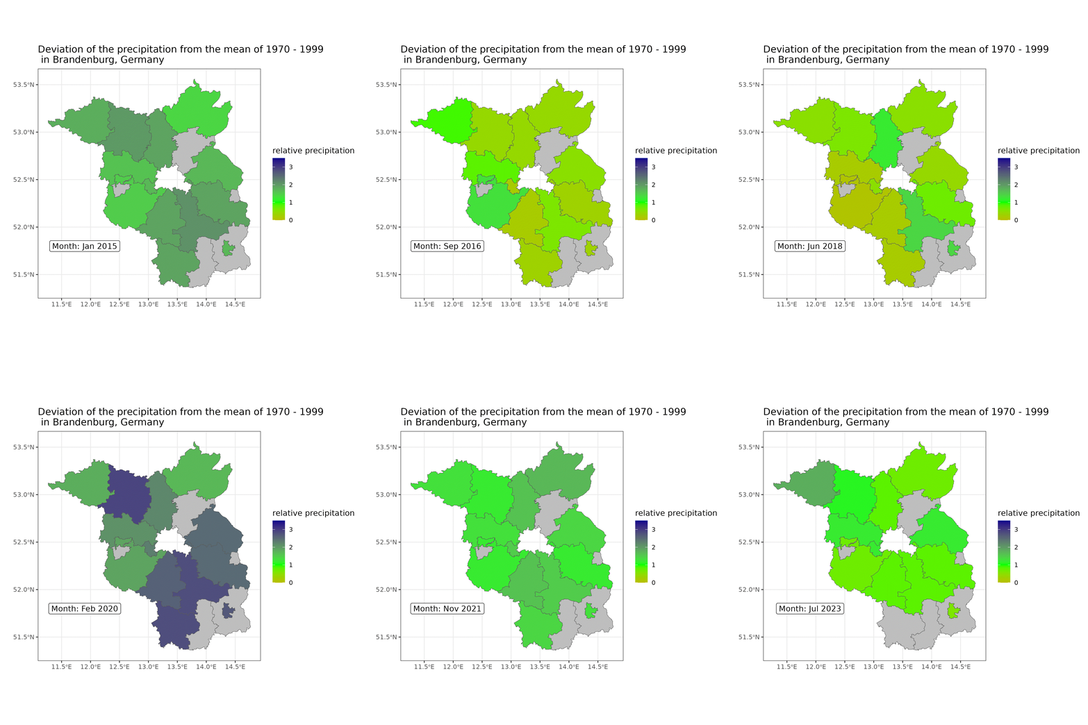Animation of the choropleth map Image description

Using the workaround results in a lower quality of the colour, which is due to the specification of the gif file format. The full source code can be found here